Given below is the T Table (also known as T-Distribution Tables or Student’s T-Table). The T Table given below contains both one-tailed T-distribution and two-tailed T-distribution, df up to 1000 and a confidence level up to 99.9%
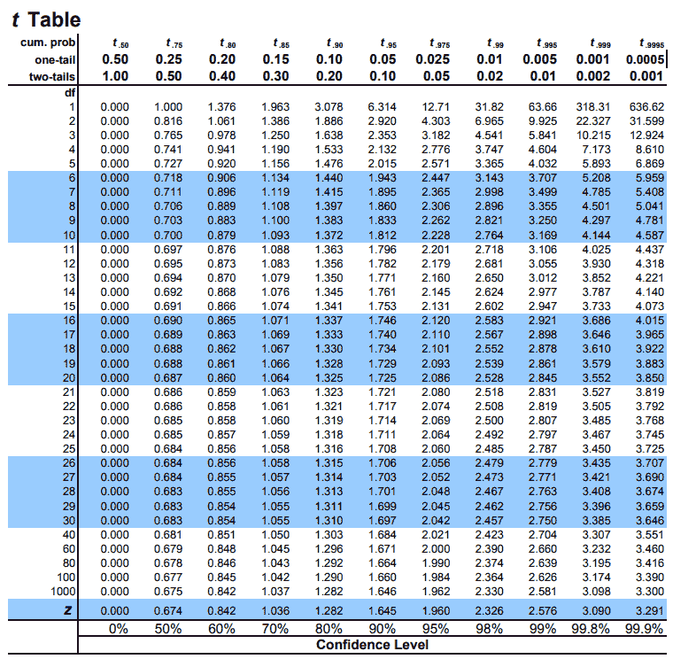
Free Usage Disclaimer: Feel free to use and share the above images of T-Table as long as you provide attribution to our site by crediting a link to https://www.tdistributiontable.com
How to Use the T-Table
Next, we are going to learn how to read the T-Table and map critical values on it using examples and diagrams but first we will need a few things or pre-requisites before we can do that.
The pre-requisites required to using a T-table are:
- The number of tails: We need to know whether our t-test is one-tailed or two-tailed because we will use the respective one-tail or two-tail row to mark the alpha level. The alpha levels are listed at top of the table (0.50, 0.25, 0.20, 0.15…for the one-tail and 1.00, 0.50, 0.40, 0.30…for the two-tails) and as you can see they vary based on whether the t-test is one-tail or two-tails.
- Degrees of freedom: The degrees of freedom (df) indicate the number of independent values that can vary in an analysis without breaking any constraints. The degrees of freedom will either be explicitly mentioned in the problem statement or if it is not explicitly mentioned, all you have to do is subtract one from your sample size (n – 1) and what you get will be your df or degrees of freedom.
- Alpha level: The alpha level ( α ), also known as the significance level is the probability of rejecting the null hypothesis when it is true. The common alpha levels for t-test are 0.01, 0.05 and 0.10
Once you have all three, all you have to do is pick the respective column for one-tail or two-tail from the table and map the intersection of the values for the degrees of freedom (df) and the alpha level.
Let us understand how to read the T-Table using an example of an one-tailed test.
Example: Let’s say we want to map an one-tailed t-test for a mean with an alpha level of 0.05. The total students involved in this study are 25. What critical value should we compare t to?
Answer:
- Firstly, we see that there are 25 students involved in this study. To get the degrees of freedom (df), we have to subtract 1 from the sample size. Therefore, df = n – 1 = 25 – 1 = 24.
2. Next, we see that our t-test is one-tailed. So we will choose the one-tail row to map our alpha level.
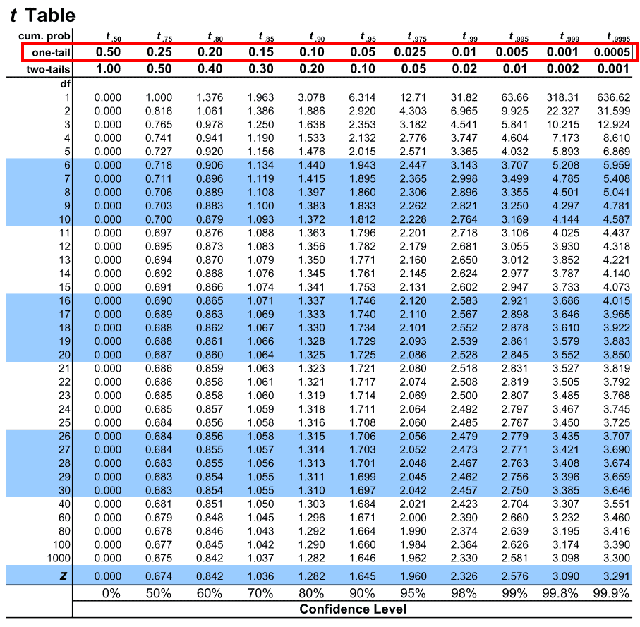
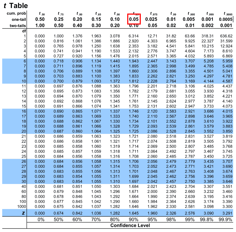
3. Next, we look for the alpha value along the above highlighted row. Our alpha level for this example is 0.05. Let us map the same on the table
4. Once that is done, let us map the degrees of freedom under the leftmost column of the table under (df)
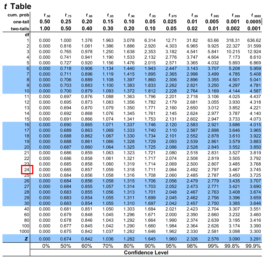
5. The intersection of these two presents us with the critical value we are looking for
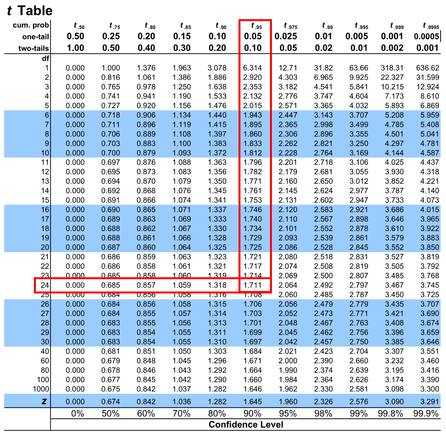
Hence we see that the critical value corresponding to our t in the t-distribution table is 1.711.
In a similar way, you can also map critical values for two-tailed tests with the only difference being that you have to select the two-tailed row of alpha values instead. The rest of the steps are the same.
Sample Questions
Following are some sample questions for your practice.
Question 1: For a two-tailed test with an alpha level of 0.30 and 18 as the sample size, what is the critical value we should compare t to?
Solution: We can deduce the following from our problem statement. The sample size is 18. Therefore the degrees of freedom ( df ) = 18 – 1 = 17. We can also see that the test is two-tailed and has an alpha level of 0.30. So on the T-Table, we map the column for two-tailed alpha values first and then map the value 0.30 across it. Then we map the value 17 under the left-most column ‘df‘ and the intersection of these two is our answer which is 1.069
Question 2: For an one-tailed test, the sample size if 23. What is the degrees of freedom?
Solution: Degrees of freedom ( df ) = n – 1 = 23 – 1 = 22
Question 3: A research study conducts an one-tailed test with an alpha level of 0.10 and a sample size of 12. What critical value should be compared to the t value obtained as the test statistic?
Solution: The sample size is 12. Hence the degrees of freedom ( df ) = 12 – 1 = 11. Mapping the alpha level across the row for one-tailed alpha values and the df of 17 on the left-side of the table, we get our critical value as 1.363
When is T Distribution used?
T Distribution is used when you have a small sample size because otherwise the T Distribution is almost identical to normal distribution with the only difference being that the T distribution curve is shorter and fatter than normal distribution curve
T Table vs Z Table vs Chi Square Table
The T distribution, Z distribution and Chi Squared distribution are few of the most commonly used probability distribution patterns and it is important to know the differences between them and when to use which distribution pattern
Usually a Z Table is used when the population standard deviation and mean are known. Whereas a T Table is used when the T score is calculated without the knowledge of the mean and the population standard deviation. Generally T Table is also preferred over the Z Table to be used when the sample size is small (N<30)
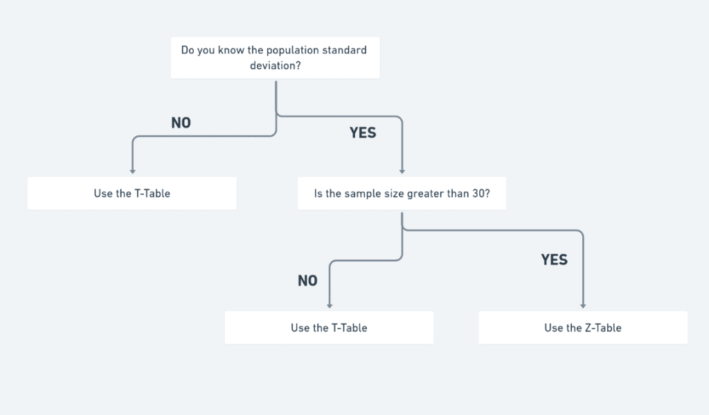
A chi square distribution on the other hand, with k degrees of freedom is the distribution of a sum of squares of k independent standard normal variables. And is used in test for the independence of two variables in a contingency table and for tests fir goodness of fit of an observed data to see if it matches to a theoretical one.
What is one tail vs two tail?
Let us understand first what a ‘tail’ is when it comes to t distribution and then let us figure out when to use a one-tailed t test vs two-tailed t test.
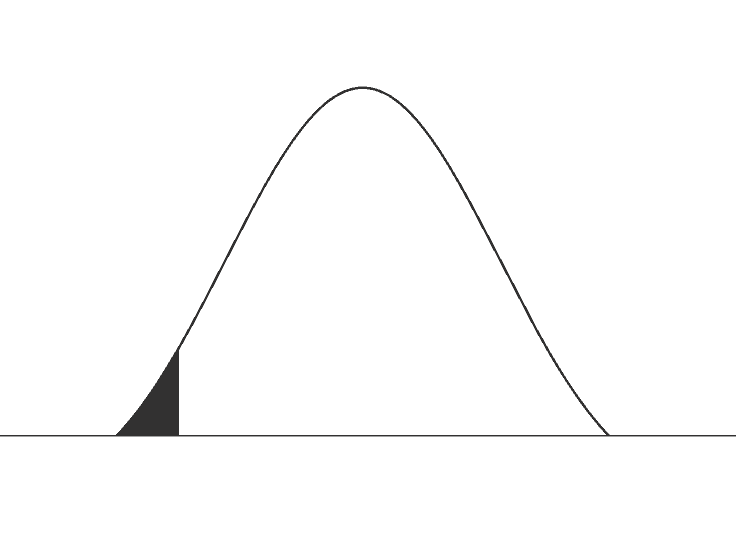
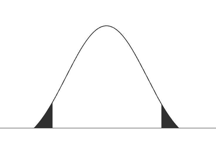
The ‘tail’ in terms of any distribution refers to end of the distribution of the test statistic. As you can see in the image alongside, the black shaded areas of the distributions are the tails. In the image where both the ends of the distribution is shaded it is said to be two-tailed and where only one end of the distribution is shaded, it is one-tailed. Usually distribution patterns like t distributions and z distributions are two tailed. Whereas asymmetrical distributions like Chi-square distributions and F distribution will have only one tail. One-tailed tests are also known as directional tests whereas two-tailed tests are also known as non-directional tests.
So how do you choose whether you want to use a one-tailed t test or a two-tailed t test? A simple way to determine that is by checking if you want to use both the negative and the positive end of the distribution (use two-tail) or if you only want to use a one directional comparison (use one-tail)
For example if you want to want to check whether Group A is both taller and shorter than Group B, then you must use a two-tailed test. Whereas if you only want to see if Group A is taller than Group B but without any interest in checking if Group A is shorter than Group B, then use a one-tailed test.
But if you are in doubt and are unsure if whether you should use a one-tailed test or a two-tailed test, then it is better to go with a two-tailed test generally.
T statistic formula or T Score formula
T statistic = (Sample mean – hypothesised mean)/sample standard error
Hence we can see that how large or how small the T statistic is depends on how close or far away the sample mean is from the hypothesised mean. If the sample mean is close to hypothesised mean, we will get a T statistic close to zero. Whereas if the sample mean if far away from the hypothesised mean, we will get a larger T statistic.
Why is T Table called as Student’s T Table or Student’s T Distribution?
The term ‘Student’ has nothing to do with the literal term student as used in the English language per se. But rather from William Sealy Gosset to whom the T-distrubtion is attributed to. William Sealy Gosset’s pen name ‘Student’ was used in 1908 to publish the distrubtion for the first time in 1908 in the paper Biometrika. The Student’s t-distribution was also initially referred to as ‘Student’s Z’ and ‘Student’s test of statistical significance’ before being commonly called Student’s t-distribution as it is known today.
History of T Table

Both the t-statistic and the t-distribution were discovered around the 19th century. T-distribution was first penned by Helmert and Lüroth in the year 1876. Friedrich Helmert born in the year 1843 in Kingdom of Saxony penned ‘Die mathematischen und physikalischen Theorieen der höheren Geodäsie’ which formed the foundation of modern Geodesy.

Jacob Lüroth born in 1844 in Germany was a mathematician known for proving Lüroth’s theorem, for introducing Lüroth quartics and his thesis on Pascal’s theorem. Although the discovery of T-distribution is credited to William Sealy Gosset, it is believed Helmert and Lüroth played a key role and derived it first. The t-distribution is also found in Karl Pearson’s 1895 paper but in a very general form known then as the Pearson Type IV.

The t-statistic however is named after and attributed to William Sealy Gosset. Gosset was born in 1876 was the Head Brewer at Guinness and is considered the father of modern British statistics. The t-statistic was introduced by William Gosset in the year 1908 under his pen name ‘Student’.
The distribution was first published in 1908 paper in Biometrika under his pseudonym ‘Student’. Hence, Student’s t-distribution gets it’s name from his pseudonym ‘Student’ and has nothing to do with the literal term student as used in the English language. The Student’s t-distribution was also initially referred to as ‘Student’s Z’ and ‘Student’s test of statistical significance’ before being commonly called Student’s t-distribution as it is known today.
Tags: T table, t distribution table, t distribution, t chart, t-table, t score calculator, t score table, t statistic, t score, t test table, t value, t value table, t table statistics, t table calculator, t-distribution table,t-distribution,t-statistic,t-chart, ttables, t tables, t chart stats, t chart statistics, t critical value, t score chart, t critical value table, student t table, full t distribution table, t-value, t test chart,student’s t table, ttable, t test, students t test,